
박가방
3. 모델링 간단 요약 - 다중 분류 (방법1, 방법2) 본문
사전 짧은 지식
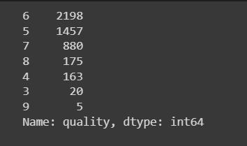
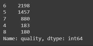
#1. data의 quality 열에서,
# 3인 경우 4로 변경
# 3이 아닌경우
# 2. 다음 data['quality']==9인 조건으로 가는데
# 9인 경우 8로 변경
# 9가 아닌 경우
# 3. data['quality']를 그대로 둔다.
data['quality'] = np.where(data['quality'] == 3, 4, np.where(data['quality'] == 9, 8, data['quality']))
이전 변경 후
1. 환경 설정
① 라이브러리
import pandas as pd
import numpy as np
import matplotlib.pyplot as plt
import seaborn as sns

from sklearn.model_selection import train_test_split
from sklearn.metrics import *
from sklearn.preprocessing import MinMaxScaler

from keras.models import Sequential
from keras.layers import Dense
from keras.backend import clear_session
from keras.optimizers import Adam
② 학습곡선함수
# 학습곡선 함수
def dl_history_plot(history):
    plt.figure(figsize=(10,6))
    plt.plot(history['loss'], label='train_err', marker = '.')
    plt.plot(history['val_loss'], label='val_err', marker = '.')

    plt.ylabel('Loss')
    plt.xlabel('Epoch')
    plt.legend()
    plt.grid()
    plt.show()
③ 파일 불러오기
path = "https://raw.githubusercontent.com----iris데이터--------.csv"
data = pd.read_csv(path)
data.head()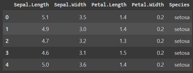
2. 데이터 전처리
- 방법 1 : y를 직접 매핑 - loss : sparse_categorical_entropy
- 방법 2 : y에 대한 핫-인코딩 - loss : categorical_entropy
① argmax에 대한 사전지식
a = np.array([[1, 2, 3], [3, 1, 2]])

# 결과 :
# array([[1, 2, 3],
       [3, 1, 2]])
# axis = 1 일 때
# axis= 0이면
# 첫번째 열의 1,3 중 인덱스 1
# 두번째 열의 2,1 중 인덱스 0
# 세번째 열의 3,2 중 인덱스 0
np.argmax(a, axis= 0)


# 결과 :
# array([1, 0, 0])
# axis = 0 일 때
# axis= 1이면
np.argmax(a, axis= 1)

# 1,2,3 중 인덱스 2
# 3,1,2 중 인덱스 0
# axis 파라미터가 없을 때
# 순서대로 인덱스가 지정됨 즉,
# 0,1,2,
# 3,4,5  <<이렇게 인덱스가 지정된 것
# 2,3인덱스 값이 3으로 동률이 있어서 인덱스 2가 나온 것.
np.argmax(a)

#결과 :
2
② 결측치 조회 - sklearn은 결측치 처리가 필수
③ y값 매핑
# y 값 매핑
data['Species'] = data['Species'].map({'setosa':0, 'versicolor':1, 'virginica':2})
data.head()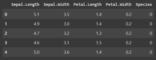
④ 데이터 정리
#target 지정
target = 'Species'

# x, y 분리
x = data.drop(target, axis = 1)
y = data.loc[:, target]
⑤ 데이터 분할
x_train, x_val, y_train, y_val = train_test_split(x, y, test_size = .3, random_state = 20)⑥ 스케일링
# Minmax스케일링
scaler = MinMaxScaler()
x_train = scaler.fit_transform(x_train)
x_val = scaler.transform(x_val)
3. 모델링
① features 선언
#num of columns
nfeatures = x_train.shape[1]
nfeatures
② 모델 구조 설계
- y 값의 범위가 0~2 이므로, 반드시 총 3개의 OutLayer 가 형성되어야 한다.
# 메모리 정리
clear_session()

# Sequential
model = Sequential([Dense(8, input_shape = (nfeatures,), activation = 'relu' ),
                    Dense(3, activation = 'softmax'  )])


# 모델요약
model.summary()
만약 OutLayer가 2개일 경우?
- softmax 식 자체가 sigmoid로 부터 유도가 됐으므로, 랜덤성으로 결과 값이 달라질 수 있지만, 비슷한 결과 값이 나올것
③ 컴파일
model.compile(optimizer=Adam(learning_rate=0.1), loss='sparse_categorical_crossentropy' )
# sparse_categorical_crossentropy - 희박한 범주형 데이터에 대한 크로스 엔트로피
④ 학습
# 학습 후, history 변수에 오차 값 할당
history = model.fit(x_train, y_train, epochs = 50, validation_split=0.2).history
⑤ 학습 곡선
dl_history_plot(history)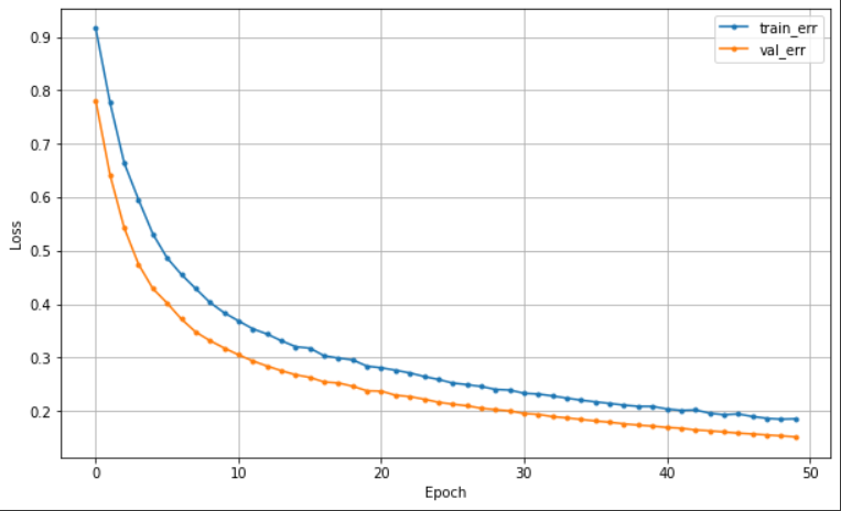
- 분명 실제 데이터와 성능은 달라질 수 있지만, 참고할 수 있는 지표다.
4. 예측 및 검증
① 모델의 예측 값을 argmax로 0,1,2로 분류
- 이유 : softmax 활성화 함수는 분류에 대한 각각의 확률을 나타내며 총합 1을 가진다.
# 설계한 model의 예측값들을 할당
pred = model.predict(x_val)
pred[:5]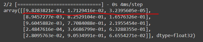
- 열은 3개의 꽃
- 행은 하나의 데이터에 대한 그 꽃에 대한 확률
- 따라서 argmax로 찾아보면 좋다.
# 전체에 적용해서 변환, 각 행중 최대 값을 가진 인덱스 추출
pred_1 = pred.argmax(axis=1)
pred_1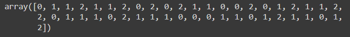
- y_val의 값도 다음과 같다. pred와 y_val의 범주가 같아졌다.
② 모델의 예측값과 실제값에 대해 confusion_matrix와 classification_report를 확인
#confusion_matrix
print(confusion_matrix(y_val, pred_1))

#classifiaction_report
print(classification_report(y_val, pred_1))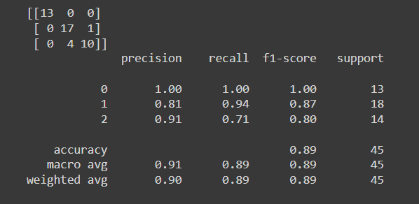
- setosa를 분류하는 건 확실한데 virginica와 2를 분류하는데에는 오류가 있구나
5. y를 one-hot Encoding 하여 설계
① 라이브러리 불러오기
from keras.utils import to_categorical② y에 대해 가변수화
 # y에 대해 가변수화
y_c = to_categorical(y.values, 3)
③ 데이터 분할
# y대신 y_c로 대체
x_train, x_val, y_train, y_val = train_test_split(x, y_c, test_size = .3, random_state = 2022)
④ 스케일링 - 딥러닝은 스케일링 필수
scaler = MinMaxScaler()
x_train = scaler.fit_transform(x_train)
x_val = scaler.transform(x_val)
⑤ 모델 설계 & 컴파일 & 학습
# 메모리 정리
clear_session()

# Sequential
model = Sequential([Dense(3, input_shape = (nfeatures,), activation = 'softmax')])

# 컴파일 - adam이 오차를 줄이는 방향으로 파라미터 업데이트.
model.compile(optimizer=Adam(learning_rate=0.1), loss='categorical_crossentropy')

#학습
history = model.fit(x_train, y_train, epochs = 100, validation_split=0.2).history
- loss가 categorical_crossentropy 다.
⑥ 학습 곡선
dl_history_plot(history)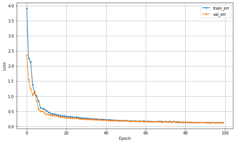
⑦ 예측값 전처리 및 할당
pred = model.predict(x_val)
pred_1 = pred.argmax(axis=1)
- one-hot encoding이 y_mapping 기법과 다른점 : 평가할 때 두 스케일(예측값, y_검증값)을 맞춰줘야 한다.
- pred_1 이 argmax에 의해 0,1,2 로 나오므로 y_val도 0,1,2로 만들어줘야 한다.
⑧ y_val 값 전처리 및 할당
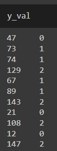
- y 값 형태 확인
#one-hot encoding된 y값 확인 - 예시
y_val[:5]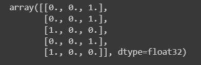
- y_val 값 0,1,2가 되도록 전처리
#y_val 전처리
y_val_1 = y_val.argmax(axis=1)
y_val_1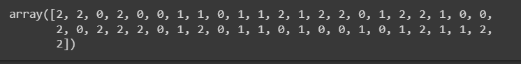
⑨ 검증
#confusion_matrix
print(confusion_matrix(y_val_1, pred_1))

#classification_report
print(classification_report(y_val_1, pred_1))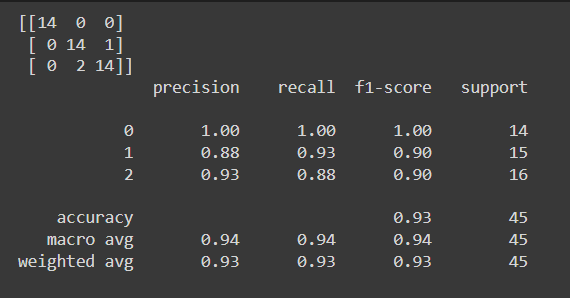
'데이터 마이닝 > 딥러닝' 카테고리의 다른 글
| fit 메소드 내 batch size (0) | 2023.03.27 |
|---|---|
| 4. Minst 손 글씨 분석[다중분류] - Early Stopping (0) | 2023.03.23 |
| 3.1 softmax (0) | 2023.03.22 |
| 2. 모델링 간단 요약 - (이진 분류) (0) | 2023.03.22 |
| 1.1 활성화 함수 Sigmoid, Relu (0) | 2023.03.22 |

